Introduction
The idea of this lab was to construct a one-degree-of-freedom helicopter, meaning the propeller is attached to a rigid piece of wood and only moves in one direction. The helicopter’s position was controlled by a python interface. The user can send input in units of degrees - the angle the helicopter’s arm makes with the ground plane.
The helicopter is controlled using a closed feedback loop. The position of the helicopter is calculated using a potentiometer connected to the helicopter’s pivot point. When the user inputs a desired fly angle, the helicopter will check its position (using the potentiometer) against the desired position and, using a PID controller, make the appropriate correction.
Design
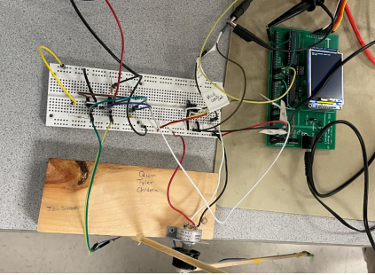
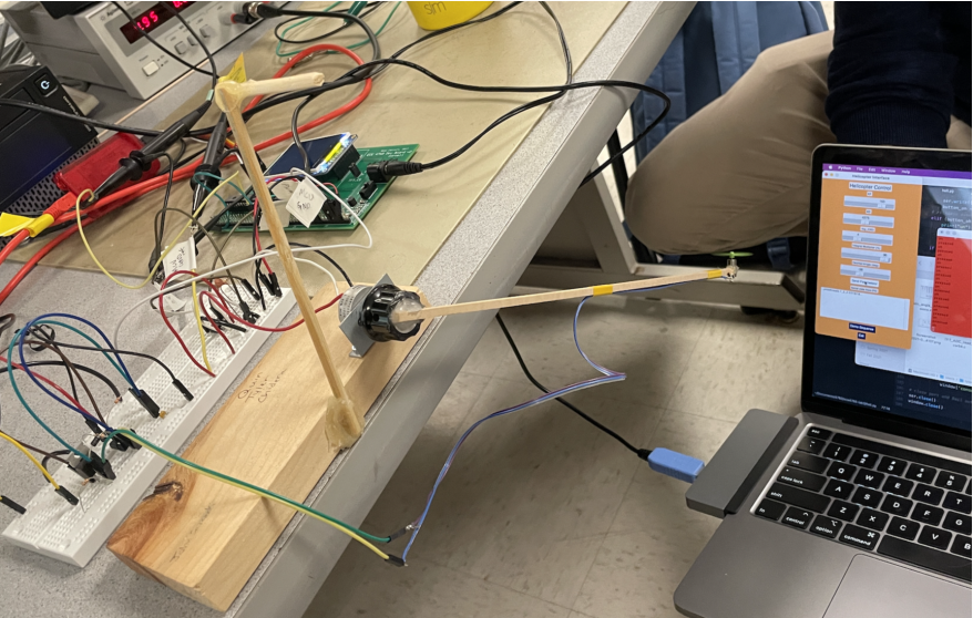
Figure 1: The Completed System
Concept
In many cases, the deployment environment of a motor is unknown, or known to have variable conditions. In these scenarios, open loop solutions that map certain conditions or parameters directly to certain outputs in a calibration stage are unreliable. For example, while the lab may have relatively stable conditions, a sufficient enough change in air viscosity or density would affect our open loop system, like weather conditions varying from week to week, or taking our system to a different location on campus or in the country. To introduce feedback and create an independent system, we need closed loop control. PID control stands for proportional, integral, derivative control, denoting the three elements of feedback going into the motor output. Proportional control acts on the current state of the system, generating output proportional to the current error. Derivative control acts on the future state of the system, generating output based on the rate of error correction. Integral control acts on the past state of the system, generating output based on the cumulative error over time. With these three elements and error reporting, we can generate a feedback loop without knowing anything about our environmental conditions. Fixing the motion of our system to one dimension makes this a much more manageable system to implement, but does not save us the issue of adapting to the nonlinear problem associated with upward thrust and gravity acting on our arm.
Hardware Description
Materials
- PIC32 + power cable
- Pickit 3 + USB cable
- TFT Display
- USB Serial dongle
- 4N35 OptoIsolator
- 1N4001 Diode
- Bench Supply (4.5V)
- 2SK4017 MOSFET
- MCP6242 opamp
- MCP4822 DAC
- 10K Potentiometer
- DC motor
Angle Sensor
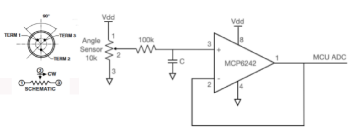
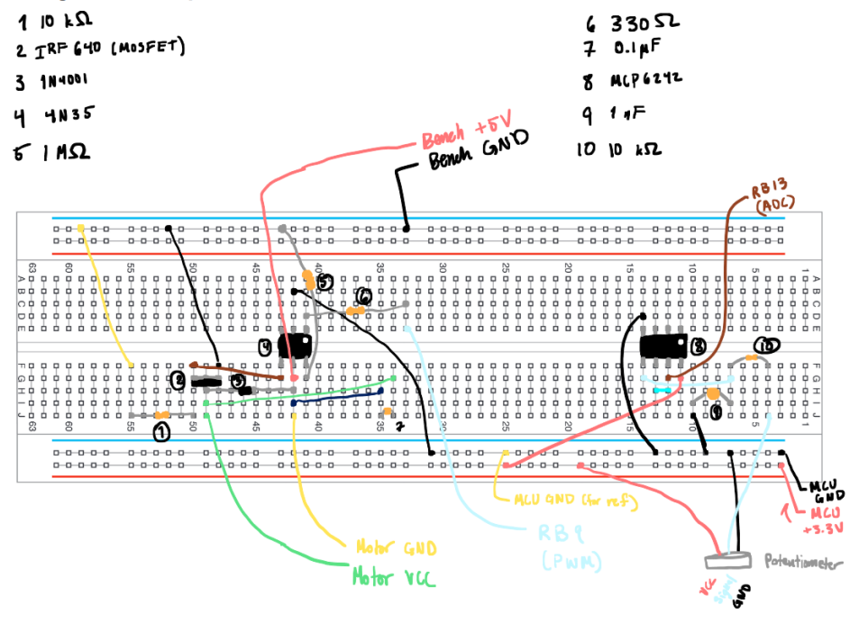
The angle sensor was an integral component of the PID controller that was used to essentially do a hardware read of the current angle value of the motor. To implement this the output terminal of 10k potentiometer tied to 3.3V and GND was connected via an anti-aliasing low-pass filter (with R and C being 100k and 1.59nF for a 1KHz sample rate) and into the input of the MCP6242 op amp which was configured as a unity gain buffer with the output being fed into the ADC of the PIC32. By tying this circuit to the ADC of the microcontroller, we were able to read the angle of the potentiometer in ADC units from the PIC. Below is a schematic of the angle sensor circuit.
Figure 2: Angle Sensor Circuit [1]
Motor
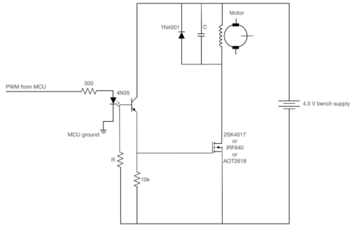
Using the instantaneous value of the ADC, the motor was sent an appropriate PWM signal that would help to mitigate the error (if any) that stemmed from the difference between a target ADC value and the current ADC value. It might be intuitive to think that one should just connect the motor directly to a pin and just send PWM signals to the motor depending on the ADC values that were read in, however, the motor circuit was designed in such a way to provide protection both to the motor itself and the PIC32 that was controlling it. Typically there are large inductive voltage spikes that can emanate from a PWM-driven DC motor. So to guard against these spikes, a 4N35 opto isolator was put in place to isolate the PIC32 from the rest of the motor circuit. In addition to that, an IN4001 flyback diode was inserted to guide any reverse-polarity spikes coming off the motor back to ground, and a capacitor in parallel with the 1N4001 to provide a path to ground for higher frequency noise stemming from the DC motor commutator reversing very quickly.
Figure 3: Motor Circuit [1]
Connections to the PIC32 (USB Serial)
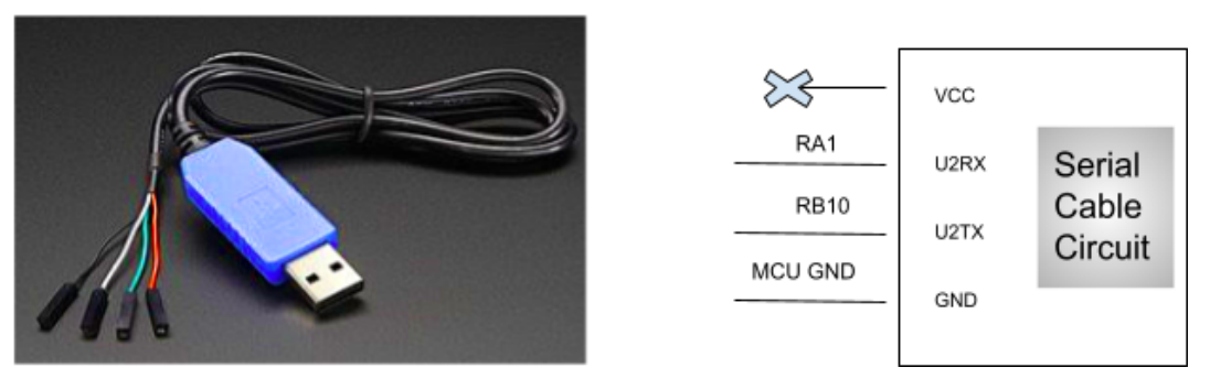
To enable a user interface so that a desiredmotor angle could be set and adjustments to the gain of the PID parameters could be communicated from a Python GUI to the PIC32 microcontroller, a UART to USB serial cable had to be connected from a computer to the PIC32 dev board. Reference Figure 4 for the schematic of the UART to USB serial cable and its connections to the dev board.
Figure 4: UART to USB Cable and Circuit
Completed Hardware Circuitry (Breadboard)
Figure 5: A Representation of the Breadboarded Hardware Connections
Completed Hardware Circuitry (Breadboard)
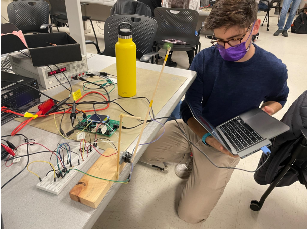
Figure 6: Helicopter In-Flight, Controlled by the Python GUI
Software Description
There are only two files that we created and worked on for this lab: Heli.c and Heli.py. The
project and clock settings in MPLab were left as default, and Bruce Land’s libraries for
protothreads and serial were used.
Heli.c
Main()
In main(), we must set up timer2 to generate the PWM signal. We want the PWM signal to run
at 1000Hz, so the period of the signal will be 40,000 clock cycles. Then, in the ISR, we do the
calculations of what the duty cycle of the PWM signal should be.
Also in main, we set up the ADC so we can convert the potentiometer voltage reading from an analog signal to a digital signal that we can actually use.
Finally, we set up DACA and DACB to be used as outputs of the system. The DACs will be fed into different channels of an oscilloscope to be used for debugging purposes. One channel will be displaying the position of the helicopter’s arm, and the other will be a windowed average of the PWM signal. The windowed average will be large if the duty cycle is large and small if the duty cycle is small. When viewing both signals at the same time we can get a sense of how the system responds with PWM outputs to different angle inputs.
Timer 2 ISR
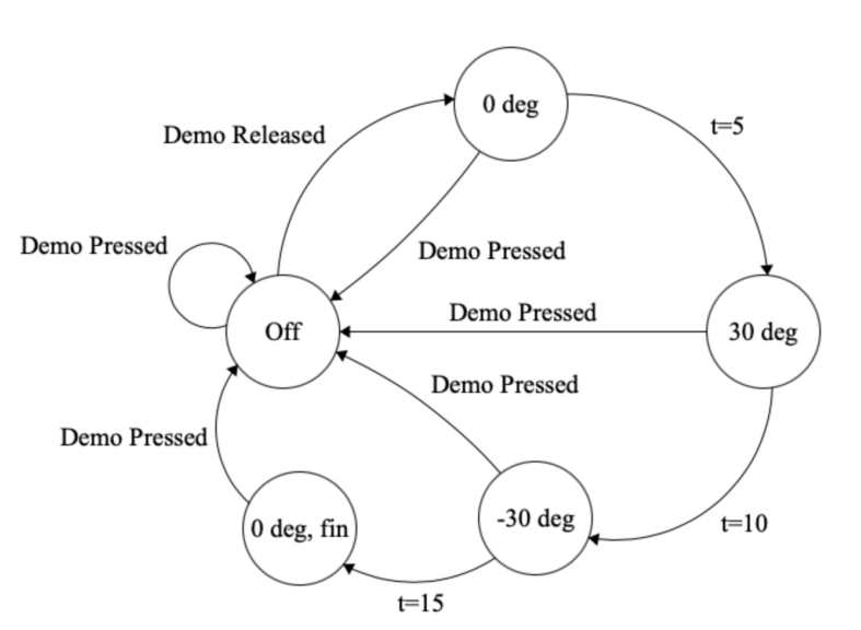
The ISR is responsible for setting the angle of the helicopter by adjusting the PWM signal. In order to handle the demo, we must move through a sequence of desired angles every five seconds. When the demo button is pressed the motor turns off. The demo commences when the button is released. The figure below describes the desired behavior of the demo states.
Figure 7: Demo FSM
In the ISR, a switch statement is used to set the desired angle and increase the number of
milliseconds since the demo was released by 1 on every time the interrupt routine is run since
the routine is run at 1000Hz. The volatile int demo_state keeps track of the state. When
we are in the finished state, the arm is set back to the horizontal position once so the demo
finishes and we can go back to manually controlling the desired angle using the python GUI.
Next in the ISR, we read the ADC and send that reading to DAC channel B so we could view
the ADC reading live on the oscilloscope. We left-shift the ADC result by 2 when sending it to
the DAC because the ADC is 10 bits but the DAC is 12 bits. This will give us a larger magnitude
to work with when viewing. On DAC channel A, we take a windowed average of the last 16
PWM duty cycles, by doing motor_disp = motor_disp + ((pwm_on_time - motor_disp) >> 4);
and then sending motor_disp to DAC A with the probes of an oscilloscope hooked up
accordingly. motor_disp is an int (16 bits), so we right-shift it by 4 to prevent overflow.
The rest of the ISR concerns itself with actually calculating the “proper” PWM signal. We use a
closed feedback loop so the system can continually check and correct itself to the proper error.
We implemented a PID controller to accomplish this goal. The three terms associated with our
PWM output at a given time are based on the proportional error, integral error, and derivative
error. We read the current angle in ADC units from the potentiometer, and take the difference
compared to the target angle in ADC units to get the angle error. Our final proportional term is
the product of a user-defined constant KP and the angle error. Our final derivative term is the
product of a user-defined constant KD and the difference between the current angle error and
the past angle error. We used the fourth previous angle error in our calculation to reduce noise,
so we update and keep track of the 4 previous angle errors in the ISR as well. Our final integral
term is the summation of all the past angle errors shifted right by a user-defined constant KI.
The final PWM signal pwm_on_time is the summation of all three of these terms, but we make
sure to clamp this value with a lower bound of 0 and an upper bound of 39,999.
So that the integral term does not accumulate an offset and destabilize the system over time, we
apply damping to the integral control. Originally, we reset the integral control on a sign change,
but this caused the arm to drop when it reached the target angle. Instead, when the sign
changes, we scale down the integral control, multiplying by inte_damp (which is equal to 0.9).
We found that this still caused the motor to drop at the target angle, at which point the arm
would be around the target angle, causing the sign of the error to switch. We added another
condition to guard against damping the control when the motor is at or around the target angle.
If all the past errors are within a certain delta of the target angle, then we should not damp the
integral control. By watching the angle reading on the TFT when the arm was stabilized at a
target angle, we decided to set delta to 3.
Serial Thread
The serial thread is responsible for waiting for input from the Python terminal and updating the
boids parameters accordingly. When the thread enters its while(1) loop, it yields inside
PT_SPAWN until the Python terminal fills the buffer with a command. For this lab, we only have
two different possible commands: a slider or a button. If the buffer receives a slider input, the
corresponding variable will be updated to whatever that input is.
The sliders are KP, KD, KI, Integral Multiplier, and Desired Angle. KI is calculated with a right
shift, so if the slider shows 4, then KI = 1 >> 4. Integral Multiplier is a percent, so in the serial
thread we divide the slider value by 100.0. Finally, the desired angle is represented in the slider
as a degree, but the PID controller only knows ADC units. Therefore, when we read a desired
angle input from the slider, we convert from angle to ADC using a linear slope. The accuracy of
this formula will be discussed in the results section.
Heli.py
Heli.py is a python script that launches a GUI to control the helicopter through a serial
connection. For this lab, the requirements for how the system must be controlled was much
looser. In our python script, we use a library called PySimpleGUI to create the GUI.
Figure 8: The Helicopter User Interface
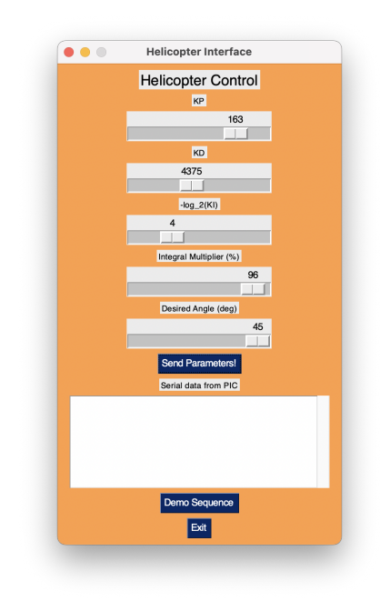
There are five sliders that the user can set. KP, KD, and -log_2(KI) impact the behavior of the
system by changing the PID controller’s parameters. As seen in Figure 8, the KI slider is set to 4. Therefore, since 4 = -log_2(KI), KI = 1/16. The reason for the decision to make the slider like
this is so a bit shift could be used for KI no matter the slider position.
The fourth slider is the integral multiplier in percent. This value is the number the integral value in the PID controller will be multiplied by every time the difference between the desired angle and the current angle has been less than two ADC units for two milliseconds. The desired angle slider is in degrees, which is most intuitive for the user. The conversion to ADC units is done inside the serial thread on the PIC, as discussed earlier.
The largest improvement to these sliders is in the ‘Send Parameters!’ button. In order to instantaneously update all of the parameters at the same time, we do not send any data to the PIC unless this button is pressed. When moving the slider, the system is not doing anything - just animating the GUI. When the button is pressed, we read the values of all five of the sliders and send all five values to the PIC.
Finally, we have a ‘Demo Sequence’ button. This button had to be a realtime button because
we must turn the motor off when the button is held and then begin the demo as soon as it is
released. Using a variable to determine whether the button is being pressed or not pressed, we
can communicate with the PIC this information. Then, depending on the state of Demo the
PIC can just follow the FSM in Figure 7 to execute the demo.
Testing
Oscilloscope
Figure 9: Oscilloscope Display of Demo Sequence
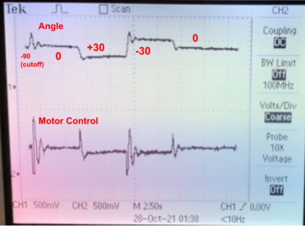
The A/B channels of the MCP4822 SPI DAC were used to display beam angle and motor
control on the oscilloscope. Using the traces on the scope we were able to test and debug if
our PWM signal and motor angles were behaving as expected. The top trace in the image
above is the actual beam angle and the bottom trace is the motor control signal used to drive
the PWM. Important to note is the fact that our potentiometer was wired in such a way that the
angle was inversely proportional to the ADC units. Therefore, the larger the ADC, the smaller
the angle. This can be seen in the figure when the voltage decreases as the angle increases to
+30º. Before displaying the motor control signal, we used a first order infinite impulse response
(IIR) filter, digital lowpass, with a time constant of about 16 PWM samples to effectively create a
PWM duty cycle averager so that the oscilloscope would display the ‘DC’ equivalent of the
PWM values that was being sent to it. The digital lowpass filter we used was given by the
following equation: motor_disp += (pwm_ontime - motor_disp) >> 4;.
Selecting P, I, and D Gains
We used the procedure recommended in the “Phenomenological Introduction to PID Controllers” by Hunter Adams to select appropriate proportional, integral, and derivative gains [2]. We systematically selected the constants, starting with proportional gain, then derivative, then integral by commanding the arm to 0 degrees (horizontal) and observing the results. We started by selecting the proportional constant on the order of 10s. On our first attempt, we increased the proportional control to get the maximum steady state error, the point at which the motor would reach the highest position without oscillating. On our second pass, we increased the proportional control to the first point at which the motor would oscillate. This was likely the reason why our first attempt at setting the constants generated unsuccessful results, whereas the second attempt did. Continuing with our procedure for the second attempt, we started with derivative control on the order of 1000s, increasing the derivative constant until the oscillation overshoot was dampened. We increased the integral control, by decreasing the integral constant as much as possible since our integral constant right shifts our integral control. We tried to minimize our integral control as much as possible, and as a final step, increased the proportional and derivative control and decreased the integral control as much as possible to achieve similar results. Our final parameters are shown below in The Final Parameters subsection of Results. The Python interface was incredibly useful in fine tuning the parameters by avoiding the need to flash a new program to the PIC to test a new configuration.
Printing
Print statements became essential for testing during this lab, both with heli.c and with heli.py. One bug was that the helicopter would not respond to angle inputs after running the demo. After printing out the desired angle to the serial monitor, it became apparent that the PIC was continuously setting the desired angle to be 400 ADC units after the demo was over. We only wanted the angle to be set once at the end of the demo to 400, not forever, and the necessary change was made to prevent this loop.
Another instance of print statements being useful was the realtime button used for demo. At first it appeared that holding down the button did not do anything and releasing the button started the demo. However, after printing the state of the button in python, it was evident that the button was triggering from 0 to 1, 0 to 1, until the button was finally released. The print statements allowed us to see that we were missing an extra condition in our if statements that would prohibit the button from toggling unless the state of the GUI actually changed.
Results
Qualitative Analysis
The inputs of the lab were the five sliders of the python interface mentioned multiple times above. The output is the behavior of the helicopter, which can be measured in terms of how stable the copter flies, how quickly it moves, how quickly it settles, and how large the steady error is at various angles.
Luckily, we were able to spend quite a while optimizing the performance of our helicopter. There
seemed to be a range of values for KP, KD, and integral multiplier that produced similarly
behaving systems. However, there was really only one KI that worked best for us given our performance goals.
We decided to prioritize minimizing steady state error and maximizing stability. That is to say, when the helicopter reaches the desired angle, it should just stay there indefinitely. We were able to achieve this at a very slight cost to the amount of time it would take for the robot to go from a very low angle to a very high angle.
The final system was extremely stable, accurate, and always damped out oscillations pretty quickly. Sometimes, it would take a few seconds to reach the desired angle, especially if the helicopter is starting out from hanging in the off position, but other than that, changes in desired angle were snappy and responsive. The system always snapped back in place if it were bumped, and would be able to correct itself even if the helicopter was held down for a while.
Quantitative Analysis
The Final Parameters
As discussed in the qualitative analysis section, there was a general range of values that
worked pretty much the same for us. Our favorite value for KI was 1/16, but a value for KP
between 150 and 160 did not change the behavior significantly enough that we needed to
fine-tune the system by analyzing the effects of changing KP by 1. The same is to be said
about KD. We found that a KD of around 5000 worked pretty well. For the final demo, we
bumped that up a bit to produce smoother oscillations. As for the integral multiplier, any value
between 90 and 100 worked perfectly. Any lower would produce some jitter from decreasing the
integral component too significantly.
Figure 10: PID Final Parameters
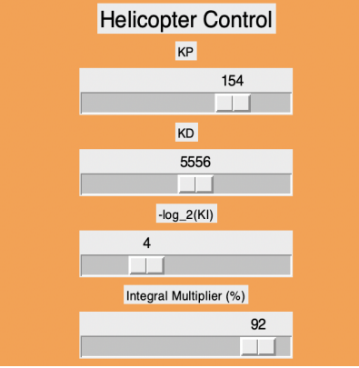
These parameters produced a robot that would snap to angles in a matter of 1 or 2 seconds. When going low to high, there are only 1-1.5 oscillations before settling. When going high to low, there are 1-2 oscillations before settling, but the first oscillation is relatively large. The steady state error at every allowable angle is negligible to the human eye.
Figure 11: Tyler Controlling and Fine-Tuning the Helicopter in Real-Time
Minimum and Maximum Angles
We decided to make 0º the horizontal which aligns with trigonometry and is therefore more intuitive to the user. Therefore, our minimum angle is -90º, when the motor is turned off. We set the maximum angle to be 45º. At 45º, the steady state error is 2º based on our angle to ADC approximation. Going past 45º gets difficult because hardly any force is required to move the motor since gravity is playing less and less of a role as the angle gets larger. Therefore, steady state oscillations get larger than what we deem acceptable as we approach 60º.
Angle to ADC Conversion
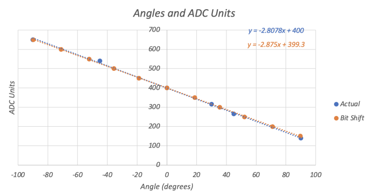
We could map a few angles to ADC units by using an iPhone’s protractor and holding the
helicopter arm. Then, we printed out the ADC value to our already-working python terminal.
Using Excel, we graphed the results. The potentiometer turned out to be linear (y = mx + b), but
the slope was -2.808. The last thing we want to do is floating point calculations, so we started
to approximate this. m = -3 was too much of an error; we were not willing to accept such an
approximation. We recognized that we could come fairly close by using just bit shifts and
adds, plus the added bonus of still being able to use an integer instead of using an Accum and
something like m = -2.8. So, m = -2.875 was chosen. With b = 400, errors were negligibly small
when the magnitude of the angle was less than 45º. As we creep into the 60-80º range, the
error grows to about 2º, which is still too small to be seen by the human eye.
Figure 12: Negligible Error Between Floating Point ADC Conversion and Bit Shift
-2.875 * ang = -ang * (2^1 + 2^-1 + 2^-2 + 2^-3)
Or, using bit shifts
-2.875 * ang = -((ang << 1) + (ang >> 1) + (ang >> 2) + (ang >> 3))
This is incredibly advantageous! We do not even need to multiply ang (desired angle in
degrees) by anything at all to convert to an ADC unit. Whenever the desired angle slider is set,
we run this inline formula and set our volatile int desired_angle in ADC units.
Conclusion
In this lab, we learned about the advantages and implementation of closed loop control. While open loop control is applicable in certain scenarios, when the deployment environment is unknown or variable, closed loop control and feedback mechanisms are highly advantageous by comparison. We incorporated a feedback loop in our system with the potentiometer, and implemented a PID controller on the PIC to control the motor. The hardware component was also more involved, and we were introduced to the considerations necessary when designing a circuit with motors and PWM control, including the need for electrical isolation between the motor and the controller to protect against back-EMF.
Ultimately, we were successful and implemented a system where a user can specify a target angle, and the motor arm will move to and maintain its position at the specified angle. The user interface allows the user to intuitively control the lever arm, specifying the angle in degrees instead of the obscure ADC units the PIC uses to describe the potentiometer position. The user can also click and press-and-hold a button to perform the demo sequence. The user can also appreciate and experiment with the aspects of PID control by easily modifying the three parameters of PID control.
Though we ultimately completed the lab in three weeks, we missed the first checkout. In a moment of oversight, we had connected our oscilloscope to RB3 and RB9 instead of the correct pins on the header, DACA and DACB. This mishap was disappointing since the rest of our hardware setup and the code were working properly and we spent a couple hours debugging a problem that did not really exist. Thankfully, we were able to quickly bounce back and stay on schedule for the second checkout.
This was not the only setback we encountered during this lab. The fine tuning of the PID constants proved to be time consuming. On our first attempt, when we were adding in our integral control, we either encountered a system that was either very slow to respond where the motor sped up gradually to leisurely meet the target angle, or a system that was too unstable and was unable to maintain the target angle. A large time sink in tuning the system was the reluctance to make a second pass at fine tuning the PID controller. We revisited the significance and effects of each of the PID terms and tried to qualitatively and deterministically adjust the system. Ultimately, we found success when we used our Python program to redefine the constants from the start of our procedure. This highlights the importance of the Python program when debugging and fine tuning the system and its usefulness in providing an efficient alternative to reprogramming the PIC with new control parameters. Additionally, when debugging systems like PID controllers that require complex tuning and trial-and-error, sometimes it is best to record the progress of the current attempt and restart.
One thing we did that other groups did not was the inclusion of a ‘send parameters’ button in the Python GUI. Other groups experienced a bug when moving their sliders too quickly because the PIC was receiving tons of slider inputs very quickly. It was described in lecture that it might be worth considering using a text box to enter the desired angle. However, a text box is not as aesthetically pleasing as a slider when attempting to display the full range of acceptable values and allowing users to slide to wherever they want. This clean look also allows the helicopter to “snap” into position as soon as new parameters are sent.
One direction we could take in continuing our investigation from this lab is improving the responsiveness of the system. For example, when the motor goes from the straight down position to the horizontal position, the arm still moves pretty slowly. Potential areas of investigation include adding nonlinear terms to our controller or another motor to the arm in the opposite direction. The motion in our system is not a linear problem with respect to the motor output. Providing a better mathematical model for the controller that takes into account pendulum physics, gravity, and air resistance and does not rely on sine-angle-approximation may produce better results. Another, less analytical approach would be to add another motor to the arm facing the opposite direction of the current motor. This would offer more control of the arm and remove the dependence on gravity to move the arm in the opposite direction. Two motors facing in the opposite direction might provide us with improved error correction. Potentially, this added control would allow us to be more aggressive with our proportional control, provide more effective derivative control, and decrease the degree of dependence on integral control.
Resources
[1] Adams, V. “PID control of a 1D helicopter” 2021. Available: https://people.ece.cornell.edu/land/courses/ece4760/labs/f2021/lab3heilcopter/Lab3/HelicopterPIC32.html, accessed November 1, 2021.
[2] Adams, V. “Phenomenological Introduction to PID controllers,” N.D. Available: https://vha3.github.io/PID/PID.html, accessed November 1, 2021.