Objective
- Build a microphone with amplifier circuit and test using Matlab
- Use a high pass filter to generate a frequency response
- Generate FFTs using the Arduino
LT Spice
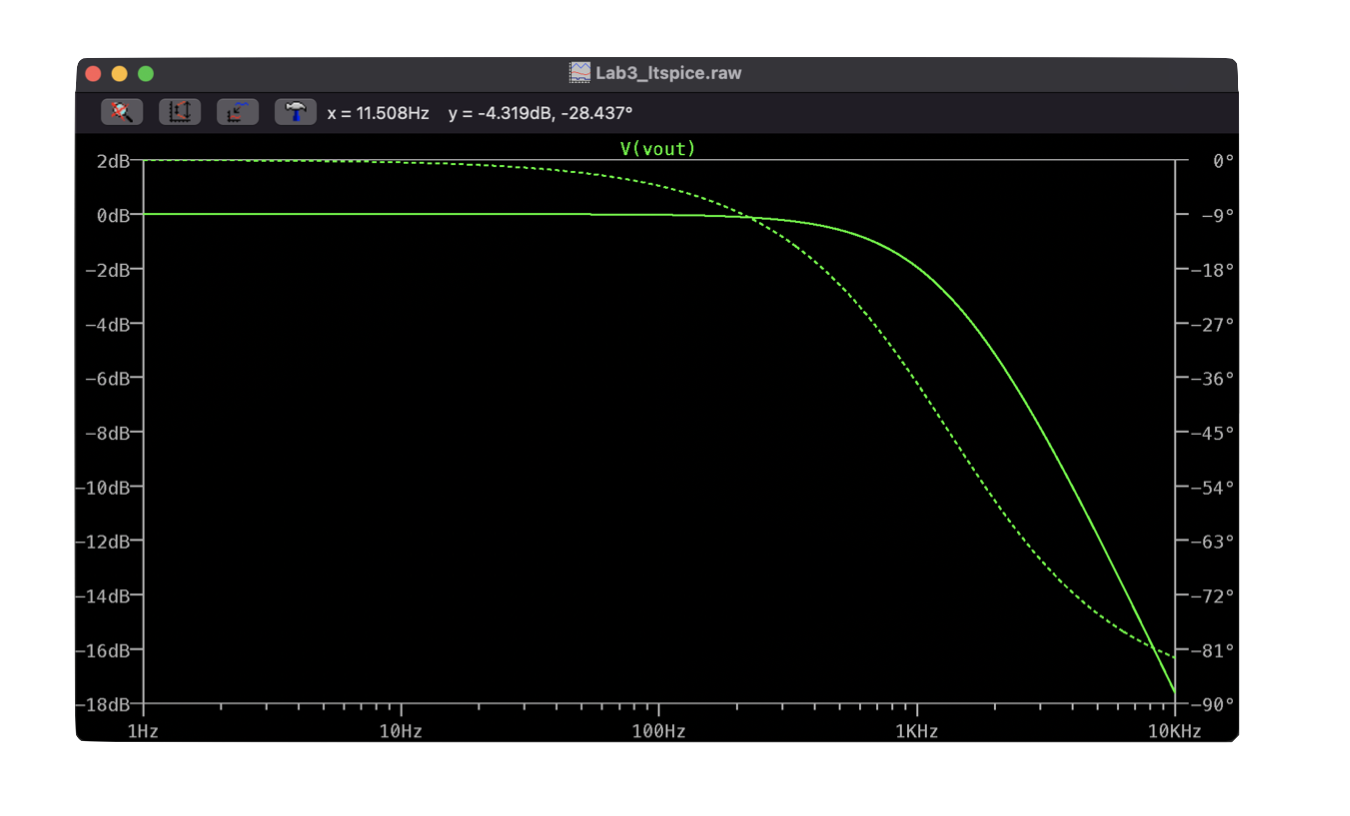
First, we built filters using LT Spice to see how an ideal, simulated filter frequency response ought to look before diving into our own. We used a 1.2 kOhm resistor and a 0.1 uF capacitor to simulate both a low and a high pass filter.
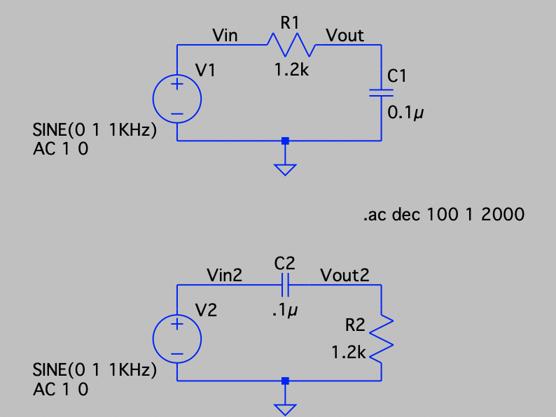
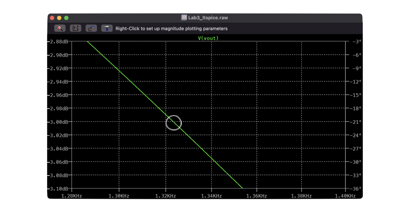
By running the circuit, we could observe the entire frequency response. After zooming in to the -3dB frequency, it was found that the cutoff freqency for both the high pass and the low pass filter was 1.32 kHz.
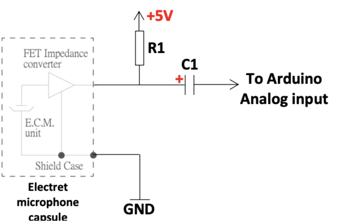
The Microphone
First, the microphone had to be breadboarded to the robot. We used pin A5 on the arduino to receive the analog signal coming out of the microphone.
Instead of doing an AnalogRead(), which can be slow, we set up the ATMega’s ADC to convert this microphone signal to a digital signal in free run mode. Then, the digital signal is sent over serial to MATLAB. The baud rate must be changed to 230400 so MATLAB can receive the microphone inputs and generate a graph of intensity vs freqeuncy. With everything connected and the correct serial port in MATLAB chosen, we then generate a 500 Hz signal while MATLAB “records” the Arduino output. The generated graph clearly shows a spike at around 500 Hz.
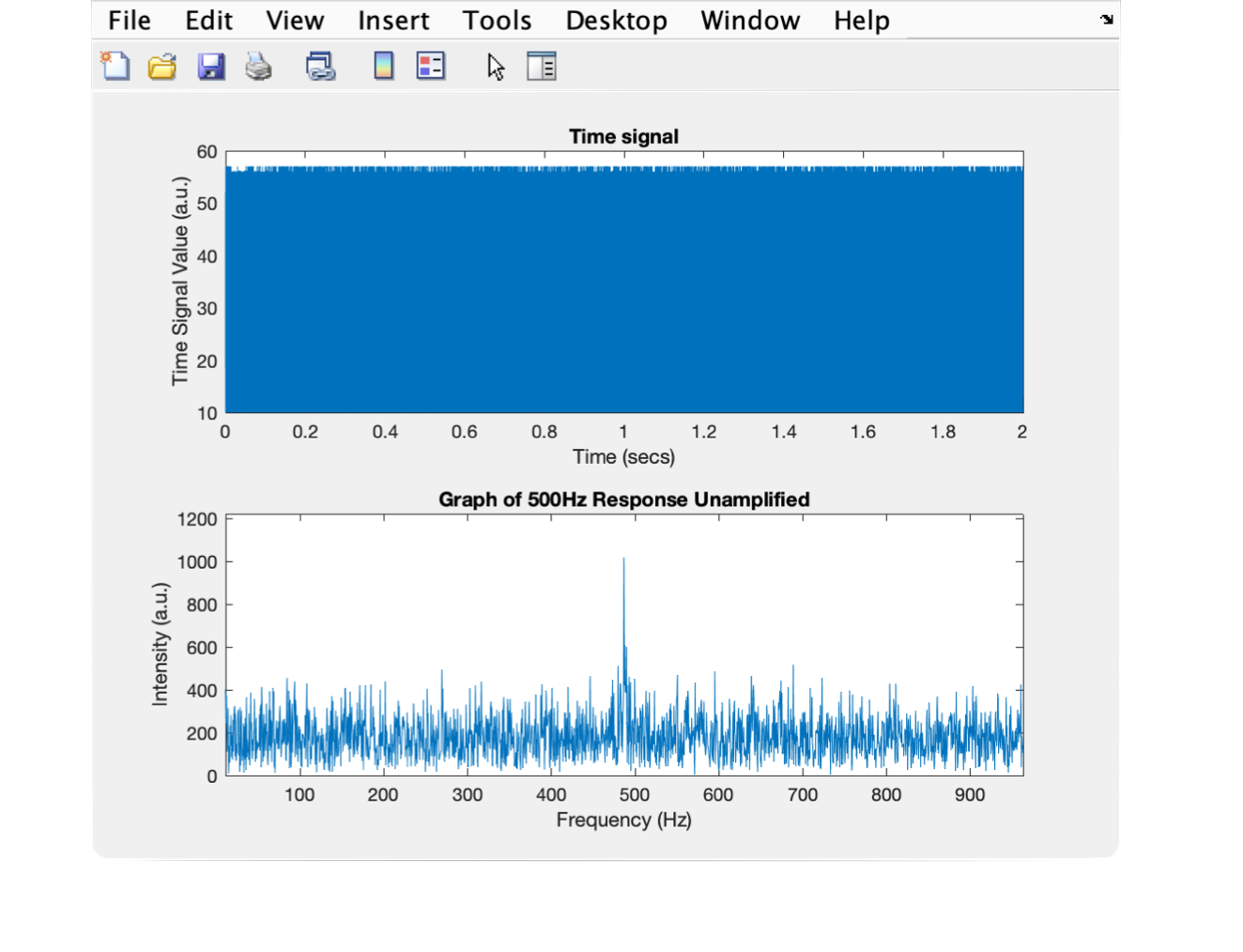
This signal is unamplified, which makes the noise to peak ratio fairly large, something that can be improved with the use of an operational amplifier.
The Amplifier
Next, an amplifier was introduced to our microphone circuit.
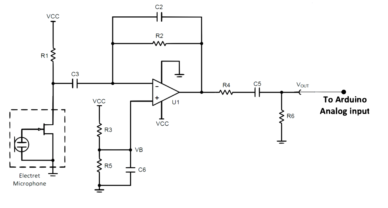
The analog pin used on the arduino remained A5, the arduino was not reflashed, and the same MATLAB script was run. However, just by amplifying the signal, the graph produced was drastically different.
Now, since the peak intensity is 10x higher than it was before, the noise at frequncies not equal to 500 Hz is so small in comparison that it can hardly be seen, resulting in a much cleaner looking graph.
The High Pass Filter
Next, we added a high pass filter to our circuit. The code on the arduino did not change, but the MATLAB script was edited to change the sound played. Instead of a constant 500 Hz signal, we would now sweep from 100Hz to 2000Hz. Picking the high pass filter parameters, with R = 22 kOhm and C = 10 nF, gets us a cutoff frequency of 723 Hz. 723 Hz is right inside the working range of our 100-2000 Hz sweep. In order to get the full frequency response H of the filter, we needed to run two sweeps: one with the filter applied (Y) and one without (X). Then, in MATLAB, H = Y./X. Then, to put it in decibles like LT Spice, H_dB = 20*log(H). Then, the smoothed H (in decibles) can finally be plotted against frequency.
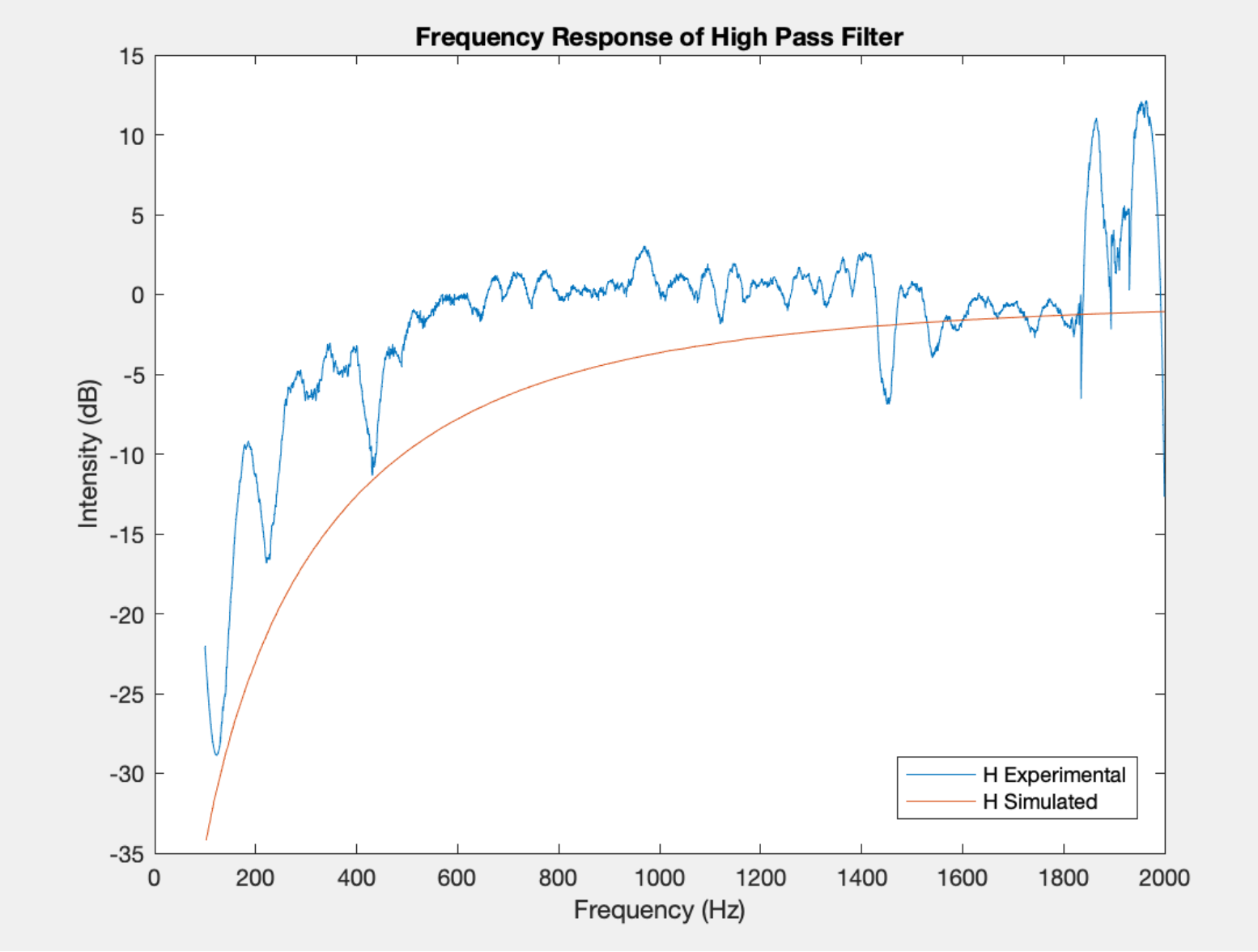
The overlay between the high pass filter simulated using LT spice and the one obtained experimentally shows that our filter is indeed behaving as expected although much less perfect and more noisy.
The FFT
For the final step of part 3, we want to generate FFTs using the arduino. Now, instead of using our ADC Freerun code that has been flashed to the Arduino since the beginning of this part, we must edit it to store FFT values.
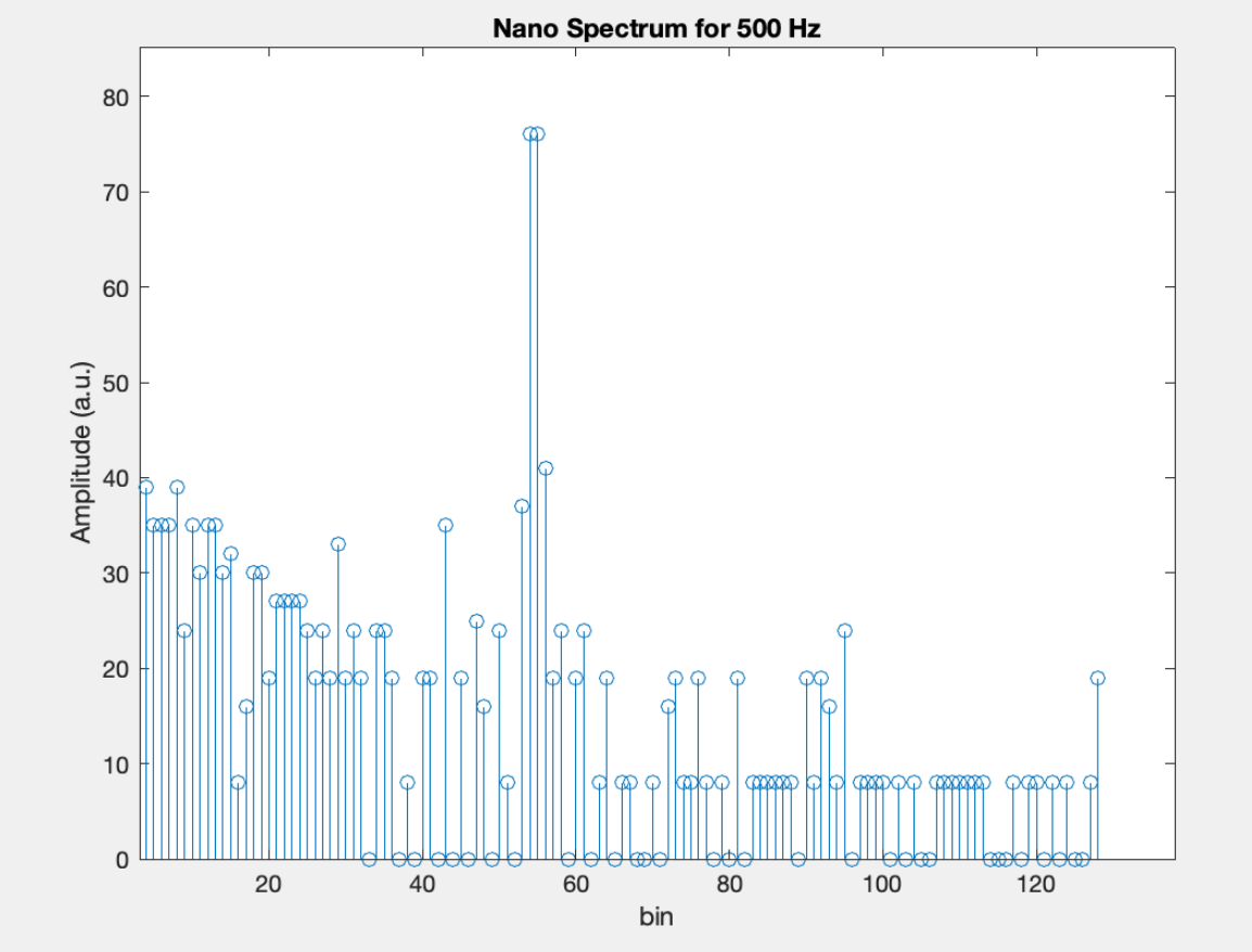
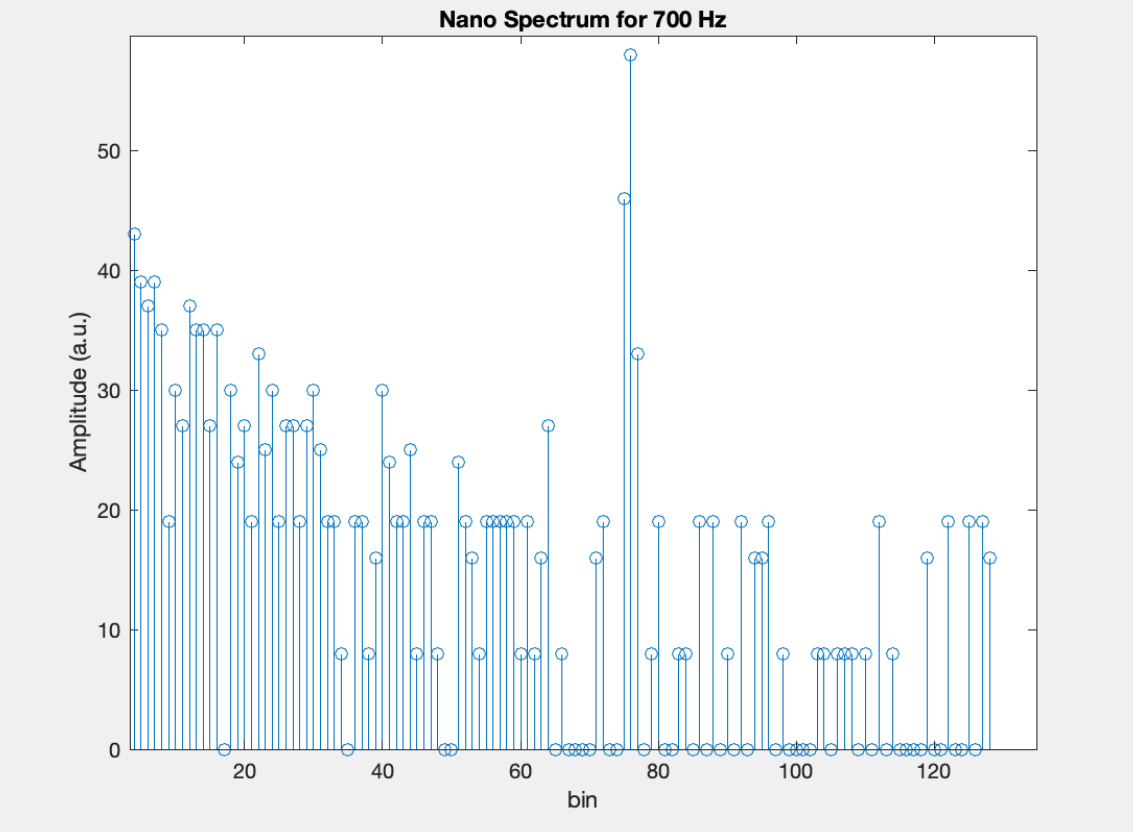
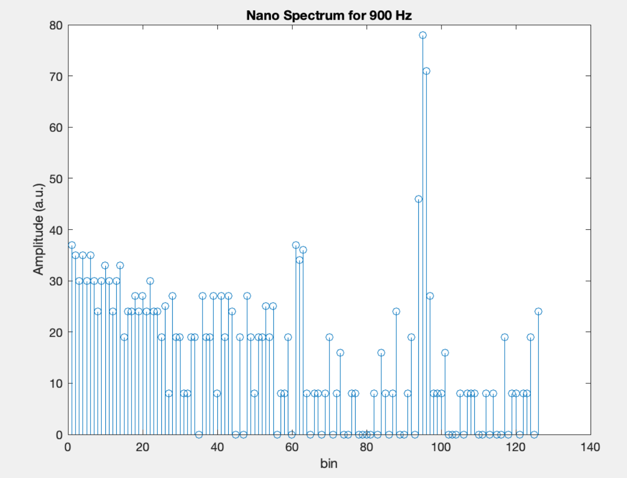
Instead of sending one ADC value at a time over to MATLAB, we must collect and store 257 samples. Therefore, we have an array and an accumulator to store the raw values from the ADC. The ADC is configured exactly as it was before: free running mode, same prescaler, etc, but instead of sampling every time the ADC is ready, we only read inside an interrupt. We configure timer interrupts to trigger on TCA0 timeout so the values do not populate too quickly. Then, our interrupt handler will read the ADC into our array and increment our counter. When enough samples have been collected, we generate an FFT. We assign an ADC value to the even entries, a zero to the odds, and throw away the first ADC value, resulting in an array of length 514. Then, using the FFT library, we use these values to generate the actual FFT. Since FFTs are symmetrical and we had produced 256 samples after throwing away the first one, we print out the first 128 entries of the FFT to the serial monitor. These printed values are the entries to our FFT, completely generated by our robot!
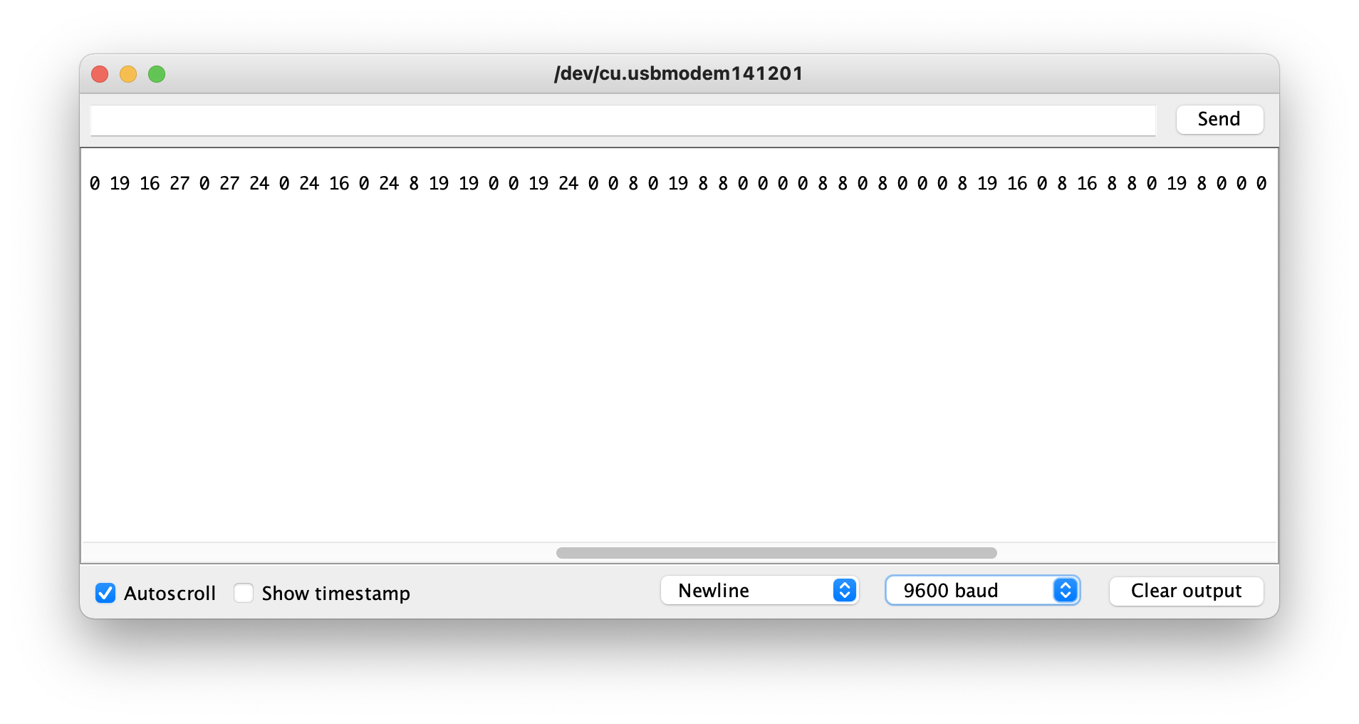
In order to graph these results to interpret them visually, we use MATLAB. By assigning the Arduino’s serial output via a copy and paste to a variable, call it y, we can run stem(y) and generate a beautiful FFT plot of the data.
The interrupts are enabled and samples are collected right when the Arduino boots up, so we must be sure to be playing a signal when the reset button on the Arduino is pressed.
Wrapping Up
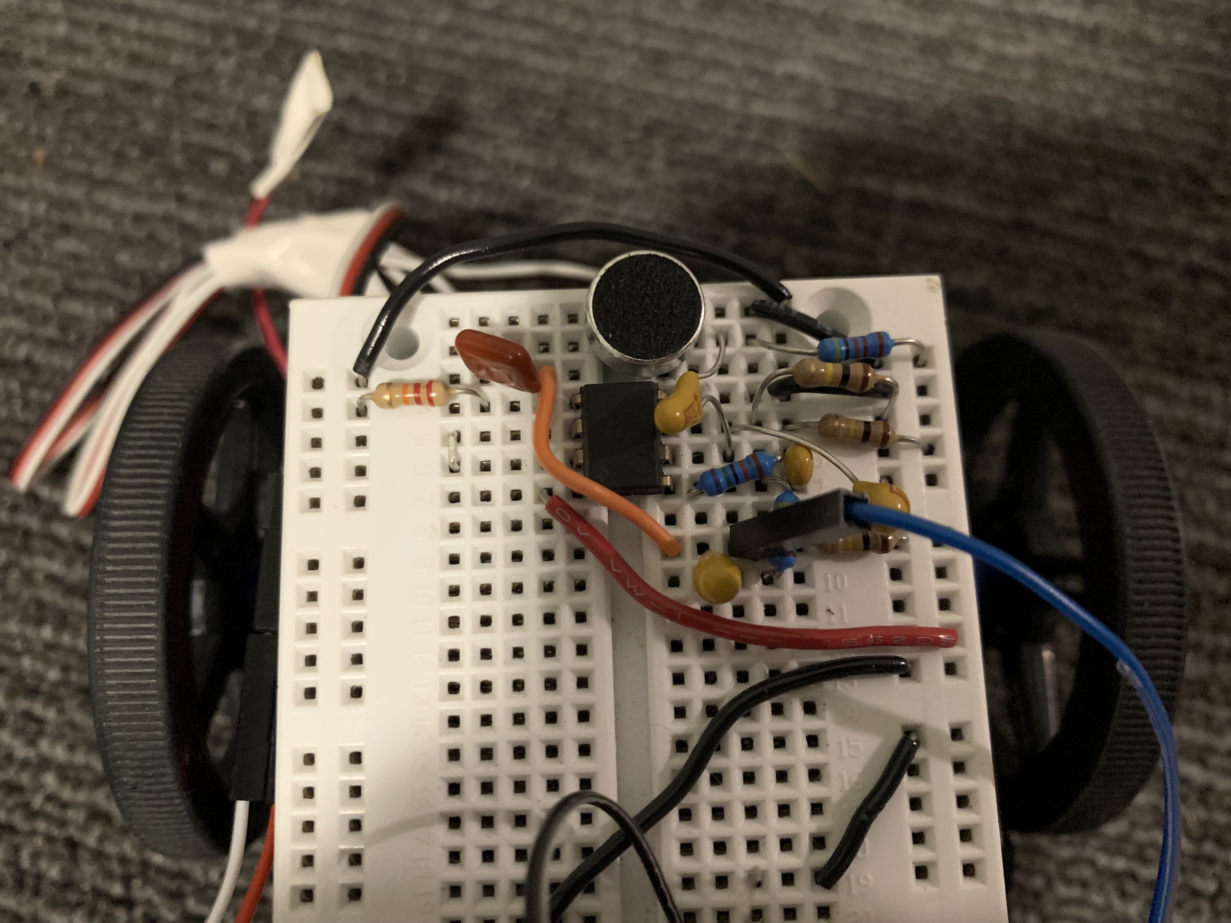
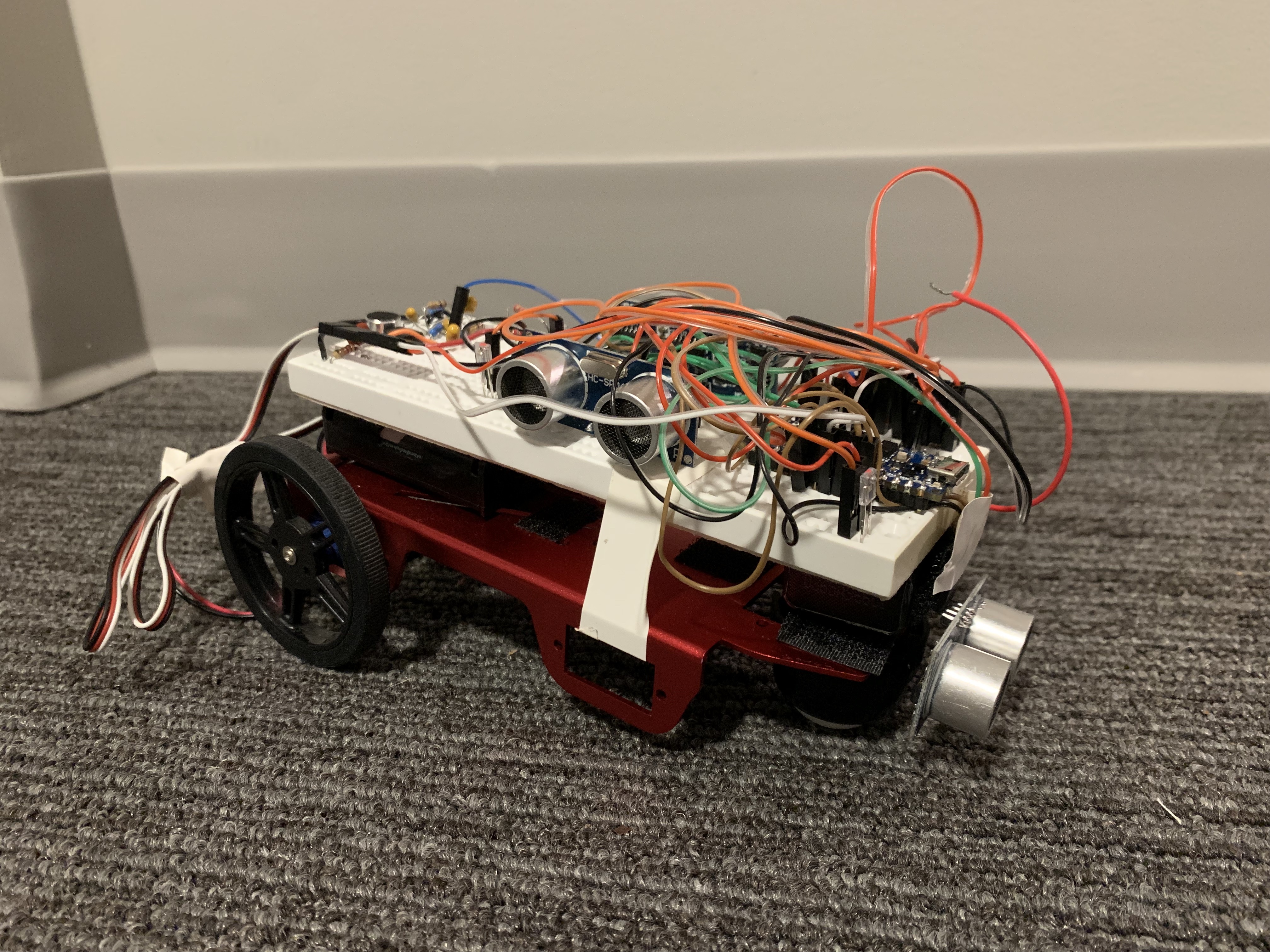
Here are a couple photos of our robot with the microphone, the amplifier, and the high pass circuitry all included.
Resources
[1] C. Poitras, Filtering & FFT, ECE 3400, October 13, 2021.